Computational models of hydrogen iodide (HI), formyl fluoride (HFCO), and p-xylene (C₈H₁₀) were analyzed using Hartree-Fock, self-consistent field computations (HF-SCF).  The basis sets that were analyzed via the General Atomic and Molecular Electronic Structure System (GAMESS) software were 3-21G, SPK-DZP, and SPKr-TZP for hydrogen iodide, and 6-21G, 6-31G, and DZV for formyl fluoride and p-xylene.  The molecular information of bond lengths and angles, vibrational frequencies, dipole moments, etc. was calculated and compared to experimental values found from the CRC Handbook of Chemistry and Physics and the National Institute of Standards and Technology web book among others.  The basis sets that calculated data closer to the experimental data were considered to be the best model used for that particular molecule regardless of the size of the basis set.  The most accurate model for hydrogen iodide was SPK-DZP and DZV for formyl fluoride and p-xylene respectively. 

Introduction

Mathematical models can very accurately calculate various characteristics of simple one-electron atoms. In that special case, the Hamiltonian term of the Schrödinger Equation for the system can be solved explicitly and quantifiable information such as the energy of the atom and the general location of the electron from the nucleus can be achieved.  Equation 1 is the general form of the Schrödinger Equation, and Equation 2 is the Hamiltonian for a one-electron atom.¹

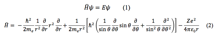
In the one-electron case, the term is completely separable, because there is no other interactions between any other particles other than the electron and the nucleus. When more electron are added to an atom, the electronic wavefunctions becomes impossible to solve since the electron-electron repulsion term prevents the electrons from being separable.  To solve for this different approximation to the many-electron atom Hamiltonian are used. The electron configuration is one of the first approximations to the many-electron wavefunction yet it doesn’t allow the distribution of one electron to change in response to the position of another electron.

 

    To obtain calculated data from more complicated atomic structures, the Hartree-Fock calculations are used.  These calculations are only possible when the Born-Oppenheimer approximation is applied.  The Born-Oppenheimer approximation states that for an atom to possess electrons, the forces between the electrons and the nucleus must be equal.  Since the forces between the electrons and nucleus are equal, the parametric qualities of the mass and acceleration must combine to offset each other.  Since the mass of a proton is at least three orders of magnitude larger than the mass of an electron, the acceleration of the electron must be equally as large to counter the nuclear mass to equalize the force between the nucleus and the electron.  In a similar fashion to the application of the center of mass relationship between the nucleus and the electrons the nucleus is so much more massive that the mass of the atom is essentially the mass of the nucleus.  Therefore since the electron has such a large acceleration vector with respect to the nucleus in any new arrangement of the nuclei, there would be an instantaneous electron response to the net electron movement.  With the Born-Oppenheimer approximation the coordinates of the nucleus and electrons are considered separable.² 

The many-electron wavefunctions calculations have more accurate results by the variational method. Variational calculations adjusts the wavefunction in order to find the minimum value for the energy of the ground state. So the lower the energy of the adjustable wavefunction, the closer is to the correct answer. Most variational methods are built initially on linear combination of atomic orbital (LCAO) with several atomic orbital wavefunction where the coefficients are the adjustable parameters in the wavefunction. In finding the expectation value for the energy, the Hartree-Fock calculation are used to approximate the electron-electron repulsion by averaging over all the positions of the other electrons. ³

   

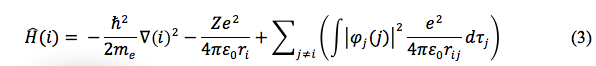
Another cornerstone to Hartree-Fock calculations is the application of Slater determinants and self-consistent field (SCF) approximations.  A Slater determinant is the use by the determinate of a matrix to evaluate the one-electron wavefunctions of the ground state configuration to generate a many electron wavefunction of an atom.  The SCF approximation is another application where the electron repulsion terms in the basis set are simplified to integrate, see Equation 3 for the general form of the multi-electron Hamiltonian.  Where the summation term shows the sum of the electron repulsion wavefunction integrals.⁴

                                                                                                                                    
 

Even with all of the approximations used: Born-Oppenheimer, Variational method, LCAO,Slater determinates, and SCF, the amount of integration required to solve the Schrödinger Equation would take an extensive length of time for only one geometry.  The use of open-sourced computational software to carry out those extensive calculations has made the amount of integration required more economical. 

 

To initiate the Hartree-Fock, self-consistent field computations (HF-SCF) for a molecule, an initial geometry of the molecule must be used.  Typically applying valence shell electron pair repulsion (VSEPR) theory using a molecular modeling software package such as Avogadro^TM is a good initial arrangement. Then that geometric data is transferred into a computational package such as The General Atomic and Molecular Electronic Structure System (GAMESS) for HF-SCF computations. 

Through those complex and repetitive calculations, the wavefunctions and nuclei of the molecule were adjusted to obtain the lowest electronic energy.  When the lowest energy was achieved, that particular geometry and other information such as vibrational frequencies, bond length, etc. were reported.  After that information was obtained, higher basis sets were used to refine the molecular properties. In these particular calculations, hydrogen iodide (HI), formyl fluoride (HFCO), and p-xylene (C₈H₁₀) were analyzed.  The basis sets used for those molecules were 3-21G, SPK-DZP, and SPKr-TZP for hydrogen iodide, and 6-21G, 6-31G, and DZV for formyl fluoride and p-xylene. 

 

From these basis set and HF-SCF computations the calculated information obtained were the bond lengths and angles, electrostatic potential maps, dipole moments, partial atomic charges, and vibrational frequencies of the respective molecules. Additionally calculated information for the molecules includes the potential energy curve for the diatomic molecule and the UV-VIS absorption peaks for the aromatic compound. All of the calculated data and other information is displayed in the various pages on this website.

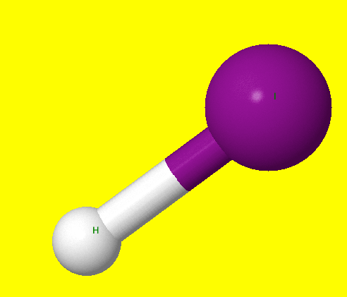
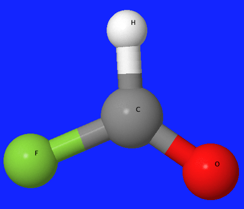
Hydrogen Iodide	Formyl Flouride	p-Xylene

Experimental

The calculations were run on mac mini with intel i7 processor and 16G of RAM. The molecules was first built using Avagadro^TM.  After the molecule was built, the file was saved and opened into wxMacMolPlt software to optimize the geometry of the molecule.  In the case of hydrogen iodide, this was not as important as hydrogen iodide is a linear diatomic molecule.  However, in the subsequent models of formyl fluoride and p-xylene, these geometry optimizations were much more important.  The purpose of the geometry optimization of the molecule is for the use in the calculations that were completed via GAMESS computation software to ensure the atoms in the molecule were appropriately spaced, thereby reducing any unnecessary calculation time. A MOPAC semi-emperical method was conducted by using either AM1 or PM3. After the geometry optimization of the molecule was completed, the lowest level of theory was used to calculate the molecular parameters for each one. Jmol was used in order to view the molecular orbitals, as well as geometry and vibrational information and visualization.

 

In the first level of theory the Huckel approximation was used.  The Huckel approximation is an initial assessment that essentially only uses the interactions between neighboring atoms in the Slater determinants that sets the remaining interactions between non-neighboring atoms to zero.  In addition, the overlap integral in the determinate was also ignored.  That left only the diagonal echelon term of the matrix that was accounted for. 

 

After the lowest level of theory was completed, in the case of hydrogen iodide this was 3-21G but for formyl flouride and p-xylene this was 6-21G gaussian basis sets, The results were  then checked to ensure that the particle exited the simulation successfully and the experimental parameters were recorded.  The end of the Hartree-Fock, self-consistent field (HF-SCF) method was then used for the next level of theory, SPK-DZP for hydrogen iodide and 6-31G for formyl flouride and p-xylene, to find a better arrangement of the nuclei.  After the calculations were completed, the new optimized geometry was used in the final level of theory.  In hydrogen iodide, that level was SPKr-TZP, in the other two molecules that was Double Zeta Valence (DZV).  The values that were calculated were then compared to experimental parameters obtained from various reference databases.  The values that were the closest to the reference databases were considered the best model used.

Conclusion

In conclusion the Hartree-Fock, self-consistent field computations (HF-SCF) is a very useful and an efficient tool to calculate molecular parameters of the three molecules when the computations were applied by the different approximations. 

 

Hydrogen Iodide

 

The SPK-DZP basis set was able to calculate the H-I bond length within 0.68% of the experimental value.  This basis set was not the largest that was used to calculate the experimental parameters, but was the closest overall in all of the calculated values compared to the experimental values.  The SPKr-TZP was the largest overall basis set used, with the 3-21G basis set being the smallest.  One possible reason why this basis set did not produce closer results to the experimental values was specifically due to the atomic size of iodine. There were 53 electrons present in the many levels of s, p, and d orbitals.  In that complexity, many of the basis sets that would have been used such as 6-21G/6-31G and DZV basis sets were not available.  However, with that complexity, HF-SCF computations were almost required to accurately discern any molecular parameters because of the amount of electrons present in the molecule.  Even with this heteronuclear diatomic, hydrogen iodide, the amount of electrons present had almost equivalent HOMO and LUMO numerical orbitals in Jmol as the polyatomic aromatic p-xylene structure.  In this particular case with the higher amount of electrons present perhaps Density Functional Theory calculations (DFT) would be slightly more accurate as DFT concentrates more on the electron density between atoms.  However, HF-SCF was still very accurate even though the complexity of electron structure due to the overall simplicity of the molecule.  With only two atoms, hydrogen and iodine, the dipole was relatively straightforward. 

 

One other important point to note with the HF-SCF calculations was the HOMO and LUMO orbital displays.  In the HOMO display, there were no anti-bonding orbitals present unlike the p-xylene molecule.  The HOMO figure illustrated the same general bond character that the MO diagram estimated. 

 

Formyl Fluoride

 

In the formyl fluoride computations, the DZV basis set was the closest to the experimental values.  In all cases, this basis set was within 1% of the experimental data obtained.  Due to this agreement between the computational and experimental data, HF-SCF calculations were very useful and applicable to the molecular structure.  Similarly to hydrogen iodide, formyl fluoride is a relatively straightforward polar molecule with a very established dipole moment.  Due to the high electronegativity in the fluorine and oxygen ends, the density of electrons at that end when compared to the more positive hydrogen side, lead to the very linear dipole moment vector.  Since this was not a complicated molecule with conflicting electronegativities, the HF-SCF showed a very good application of various parameters calculated. 

 

As stated in the hydrogen iodide molecule section, perhaps DFT would show a slightly better agreement between the calculated and the experimental reference data, but with such a low deviation, it would seem that the HF-SCF calculations were perfectly applicable.

 

p-Xylene

 

In the p-xylene simulation, this would almost require HF-SCF calculations at the very least to determine any of the parameters. As the amount of atoms increased and also due to the complexity of the aromatic structure, the modeling of this molecule was essential. 

 

In the electrostatic potential map based on these calculations, the strongest regions of electron density was inside the conjugated double bonds of the aromatic ring which is qualitatively where it would be expected from any line angle diagram of the molecule. 

 

In the HOMO display, there was such complexity in the aromatic region, that the visualization of anti-bonding and bonding character was present.  Specifically with this model, potentially DFT would have been a more accurate basis set for calculation given the higher electron density centered in the aromatic ring. 

 

In general, the molecular properties calculated illustrated very clear results that are very applicable to the three molecules analyzed.  The electrostatic potential maps of the three molecules show the locations of relative electron density.  Those regions then show the possibility of nucleophilic attraction to a more relatively positive region of a different molecule in a nucleophile addition or substitution reaction.  As the complexity of the different molecules increased, DFT may have been a better model to simulate the molecular structures

Refrences 

1. Cooksey, A. Quantum Chemistry; Pearson: New York, 2014; Vol. 1, p 148.
2. Cooksey, A. Quantum Chemistry; Pearson: New York, 2014; Vol. 1, p 211-212.
3. Cooksey, A. Quantum Chemistry; Pearson: New York, 2014;  Vol. 1, p 194-195
4.Cooksey, A. Quantum Chemistry; Pearson: New York, 2014;Vol. 1, p 174-175.

Using directory /Users/student/Documents/Jaime_Andy/WEBSITE/Introduction/Introduction Page
  adding JmolPopIn.js
  ...jmolApplet0
      ...adding Hydrogen_Iodide_.png
copying and unzipping jsmol.zip directory into /Users/student/Documents/Jaime_Andy/WEBSITE/Introduction/Introduction Page
      ...copying
file:/Users/student/Documents/Jaime_Andy/HI/HI-SPK-DZP.log
         to
      ...compressing large data file to
/Users/student/Documents/Jaime_Andy/WEBSITE/Introduction/Introduction Page/HI-SPK-DZP.log.gz
/Users/student/Documents/Jaime_Andy/WEBSITE/Introduction/Introduction Page/HI-SPK-DZP.log.gz
      ...adding Hydrogen_Iodide_.spt
  ...jmolApplet1
      ...adding Formyl_Fluoride.png
copying and unzipping jsmol.zip directory into /Users/student/Documents/Jaime_Andy/WEBSITE/Introduction/Introduction Page
      ...copying
file:/Users/student/Documents/Jaime_Andy/HFCO/HFCO-DZV.log
         to
/Users/student/Documents/Jaime_Andy/WEBSITE/Introduction/Introduction Page/HFCO-DZV.log
      ...adding Formyl_Fluoride.spt
  ...jmolApplet2
      ...adding p-Xylene.png
copying and unzipping jsmol.zip directory into /Users/student/Documents/Jaime_Andy/WEBSITE/Introduction/Introduction Page
      ...copying
file:/Users/student/Documents/Jaime_Andy/p-Xylene/PXYLENE-DZV.log
         to
      ...compressing large data file to
/Users/student/Documents/Jaime_Andy/WEBSITE/Introduction/Introduction Page/PXYLENE-DZV.log.gz
/Users/student/Documents/Jaime_Andy/WEBSITE/Introduction/Introduction Page/PXYLENE-DZV.log.gz
      ...adding p-Xylene.spt