Once the molecule file is fully loaded, the image at right will become live. At that time the "activate 3-D" icon ![]() will disappear.
will disappear.
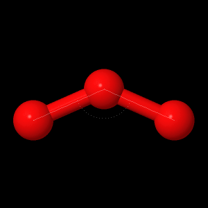
Ozone (O3)
The molecular geometry of ozone was calculated using two
semi-empirical methods (AM1 and PM3) as well as the ab initio HF-SCF
method with three different basis sets (6-21G, 6-31G, and DZV). For the
DZV geometry optimization calculation, one was done using the RHF method
and one was done using the UHF method. Table 1: Molecular geometries, dipole moments, and energies for ozone from each calculation as well as the literature values.
| Ozone | Dipole (Debye) | Bond length (Å) | Bond angle (°) | Energy (Hartree) |
| AM1 (RHF) | 1.151247 | 1.16 | 120.9 | -35.0736 |
| AM1 (UHF) | 0.636197 | 1.25 | 118.7 | -35.0260 |
| PM3 (RHF) | 1.140444 | 1.22 | 114.0 | -32.1024 |
| PM3 (UHF) | 1.107291 | 1.25 | 118.7 | -30.0489 |
| 6-21G (RHF) | 0.720246 | 1.31 | 117.3 | -223.9051 |
| 6-21G (UHF) | 0.423276 | 1.31 | 117.3 | -233.9321 |
| 6-31G (RHF) | 0.556568 | 1.25 | 119.6 | -244.1386 |
| 6-31G (UHF) | 0.462442 | 1.32 | 132.6 | -224.1535 |
| DZV (RHF) | 0.689765 | 1.26 | 119.7 | -224.2084 |
| DZV (UHF) | 0.482295 | 1.32 | 132.1 | -224.2249 |
| Literature | 0.534(5) | 1.2716(5) | 117.47(5) | ------ |
Table 1 shows that DZV UHF gave the most energetically favorable molecular geometry. However, this geometry is not consistent with the literature values. The DZV RHF method is closer for the bond length value. The 6-21G method gives the bond angle closest to the literature value, and the 6-31G RHF method gives the dipole moment value that is closest to the literature value. UHF was expected to give better values overall, as it takes into account the two unpaired electrons that ozone is known to have. Selecting the triplet multiplicity also yielded a lower energy overall, also as a result of the two unpaired electrons.
Molecular orbitals were also calculated in the geometry optimization. The molecular geometry, as well as the HOMO and LUMO for the DZV calculation can be viewed below. The HOMO was determined by filling orbitals starting with the lowest energy orbital and selecting the highest energy occupied orbital. The LUMO was determined by taking the lowest energy orbital that was not occupied by electrons.
Though ozone contains three atoms of same element, the charge distribution is not uniform throughout the molecule, largely as a result of the unpaired electrons. The partial atomic charges associated with each atom can be viewed below.
The electrostaic potential map of the molecule can be viewed below. Red indicates regions of high electron density and therefore a partial negative charge. Blue indicates a region of low electron density and therefore a partial positive charge.
Vibrational frequencies for ozone were calculated using the DZV optimized geometry. The ROHF method was needed to produce numbers that made sense. The bending frequency was found to be -2264 cm-1. The fact that it is a negative value is likely due to an error in the calculation program, though a positive frequency of the same magnitude would be a plausible value for the bending frequency. The symmetric stretch frequency was calculated to be 3704.94 cm-1, and the asymmetric stretch was calculated to be 3886.66 cm-1.
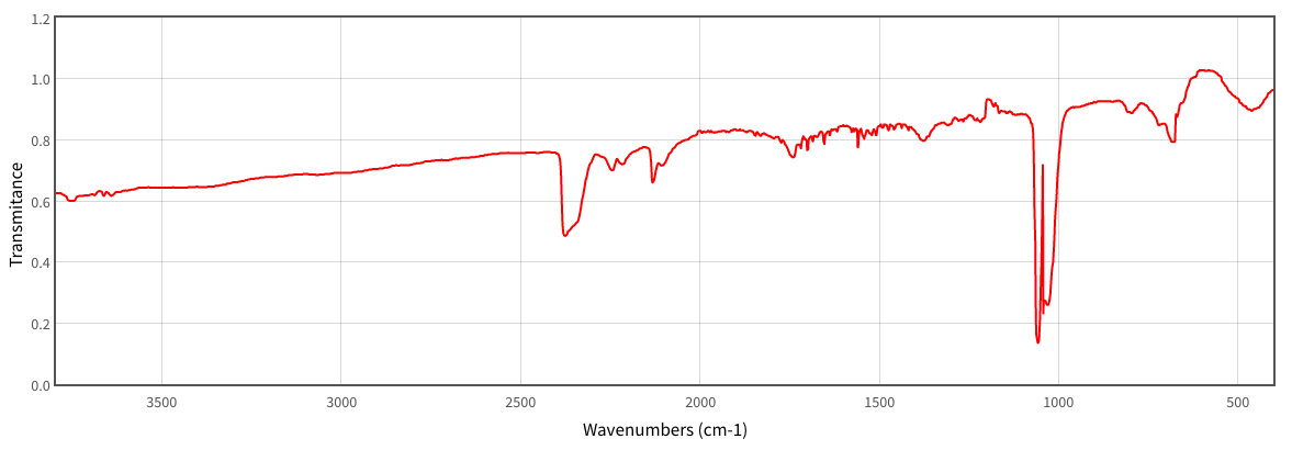
Figure 2: IR spectrum for ozone(6).
Page skeleton and JavaScript generated by export to web function using Jmol 14.2.15_2015.07.09 2015-07-09 22:22 on Feb 26, 2018.
This will be the viewer