A web page containing Jmol applets

Chlorine Monofluoride (FCl)

The MO Calculations for Chlorine Monofluoride (FCl)

	Jmol0 will appear here.
	CLICK IMAGE TO ACTIVATE 3D Figure 1: Geometry of FCl using 6-21G calculation

For Chlorine Monofluoride, the over all best calculated dipole moment was from AM1 calculation while the best calculated dipole moment among the ab initio theory calculation was 621G. The same pattern holds true for the bond length. The 6-21G calculation yielded an 28.5% error for the dipole moment and a 3.79% error for the bond length for Chlorine Monofluoride. The data collected from the calculations is shown below.

Table 1: Dipole moment and bond length for the five levels of theory.

Theory	Dipole Moment (Db)	Percent Error (%)	Bond Length (nm)	Percent Error (%)
Literature	0.881±.002 ⁵	---	.16283 ⁶	---
AM1	0.856872	2.74	0.165	1.33
PM3	1.680765	90.8	0.158	2.97
6-21G	1.132491	28.5	0.169	3.79
6-31G	1.607802	82.5	0.171	5.01
DZV	1.841146	109.	0.172	5.63

It is obvious that the results of the dipole moment and bond length from AM1 was the closest to the literature value. However, for ab initio theory, 6-21G had the closest results to the literature value. Therefore, we adopted 6-21G for the rest of the calculations for Chlorine Monofluoride.

The geometry of chlorine fluoride under 6-21G, 6-31G, DZV, and AM1 are shown from Figure 1 to Figure 4. The bond length is labeled in each figure as well. The bond angle of FCl was not included since it is 180 degrees.

Jmol1 will appear here.

Jmol2 will appear here.

Jmol3 will appear here.

CLICK IMAGE TO ACTIVATE 3D
Figure 2: Geometry of FCl using 6-31G calculation

CLICK IMAGE TO ACTIVATE 3D
Figure 3: Geometry of FCl using DZV calculation

CLICK IMAGE TO ACTIVATE 3D
Figure 4: Geometry of FCl using AM1 calculation

The Highest Occupied Molecular Orbital (HOMO) was found at orbital 13. The HOMO was calculated by dividing the sum of the total number of electrons in the molecule by 2. The Lowest Unoccupied Molecular Orbital (LUMO) was found at orbital 14. The LUMO was the orbital that would be filled by the excited valence electron(s) from the HOMO if proper excitation occurs.

Jmol4 will appear here.

Jmol5 will appear here.

CLICK IMAGE TO ACTIVATE 3D
Figure 5: Highest Occupied Molecular Orbital for FCl using 6-21G calculation

CLICK IMAGE TO ACTIVATE 3D
Figure 6: Lowest Unoccupied Molecular Orbital for FCl using 6-21G calculation

        The electrostatic potential of FCl using 6-21G calculation was shown in Figure 7. The electrostatic potential used a color spectrum, which uses red to indicate the lowest electrostatic potential and blue to indicate the highest electrostatic potential. ⁷ The electrostatic potential shows the electron distribution in the molecules. ⁷

        The partial atomic charge is shown in Figure 8. It is the distribution by the asymmetric scatter of the electrons in the molecule. Fluorine is more electronegative than chlorine. Therefore, the fluorine had the negative partial atomic charge; the electrons are more likely to hanging around fluorine.

        Since FCl is a diatomic molecule, there is only one kind of stretching possible. This is shown in Figure 9.

Jmol6 will appear here.

Jmol7 will appear here.

Jmol8 will appear here.

CLICK IMAGE TO ACTIVATE 3D
Figure 7: Electrostatic Potential for FCl using 6-21G calculation

CLICK IMAGE TO ACTIVATE 3D
Figure 8: Partial Atomic Charge for FCl using 6-21G calculation

CLICK IMAGE TO ACTIVATE 3D
Figure 9: Bond Stretch for FCl using 6-21G calculation

The valence energy level diagrams corresponding to the type of bonding occurring at specific levels is shown below in Table 2.

Table 2: Valence energy level diagrams corresponding to the type of bonding occurring at specific levels

Jmol9 will appear here.

Jmol10 will appear here.

Jmol11 will appear here.

Jmol15 will appear here.

S sigma bonding

S sigma anti-bonding

Px bonding

Px anti-bonding

Jmol12 will appear here.

Jmol14 will appear here.

Jmol13 will appear here.

Jmol5 will appear here.

Py bonding

Py anti-bonding

P sigma bonding

P sigma anti-bonding

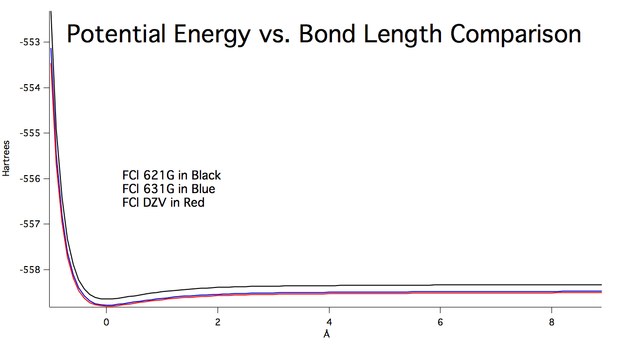
The following graph, Figure 10, shows the relationship between potential energy and bond length using different calculations.

Figure 10: Potential energy curves at different levels of theory. The graph was generated by IGOR Pro.

Based on template by A. Herráez as modified by J. Gutow

Page skeleton and JavaScript generated by export to web function using Jmol 14.2.12_2015.01.22 2015-01-22 21:48 on Mar 9, 2015.

Using directory /Users/student/Desktop/Barb and Yuqi MO/Web HTML/FCl/FCL 2/fcl 2
  adding JmolPopIn.js
  ...jmolApplet0
      ...adding FCL_6.png
copying and unzipping jsmol.zip directory into /Users/student/Desktop/Barb and Yuqi MO/Web HTML/FCl/FCL 2/fcl 2
      ...copying
file:/Users/student/Desktop/Barb and Yuqi MO/FCl/FCl_621G_opt.log
         to
/Users/student/Desktop/Barb and Yuqi MO/Web HTML/FCl/FCL 2/fcl 2/FCl_621G_opt.log
      ...adding FCL_6.spt
  ...jmolApplet1
      ...adding FCL_31.png
copying and unzipping jsmol.zip directory into /Users/student/Desktop/Barb and Yuqi MO/Web HTML/FCl/FCL 2/fcl 2
      ...copying
file:/Users/student/Desktop/Barb and Yuqi MO/FCl/FCl_631G_opt.log
         to
/Users/student/Desktop/Barb and Yuqi MO/Web HTML/FCl/FCL 2/fcl 2/FCl_631G_opt.log
      ...adding FCL_31.spt
  ...jmolApplet2
      ...adding FCL_DZV.png
copying and unzipping jsmol.zip directory into /Users/student/Desktop/Barb and Yuqi MO/Web HTML/FCl/FCL 2/fcl 2
      ...copying
file:/Users/student/Desktop/Barb and Yuqi MO/FCl/FCl_DZV_opt.log
         to
/Users/student/Desktop/Barb and Yuqi MO/Web HTML/FCl/FCL 2/fcl 2/FCl_DZV_opt.log
      ...adding FCL_DZV.spt
  ...jmolApplet3
      ...adding FCL_AM1.png
copying and unzipping jsmol.zip directory into /Users/student/Desktop/Barb and Yuqi MO/Web HTML/FCl/FCL 2/fcl 2
      ...copying
file:/Users/student/Desktop/Barb and Yuqi MO/FCl/FCl_AM1_opt.log
         to
/Users/student/Desktop/Barb and Yuqi MO/Web HTML/FCl/FCL 2/fcl 2/FCl_AM1_opt.log
      ...adding FCL_AM1.spt
  ...jmolApplet4
      ...adding FCL_HOMO.png
copying and unzipping jsmol.zip directory into /Users/student/Desktop/Barb and Yuqi MO/Web HTML/FCl/FCL 2/fcl 2
      ...adding FCL_HOMO.spt
  ...jmolApplet5
      ...adding FCL_LUMO.png
copying and unzipping jsmol.zip directory into /Users/student/Desktop/Barb and Yuqi MO/Web HTML/FCl/FCL 2/fcl 2
      ...adding FCL_LUMO.spt
  ...jmolApplet6
      ...adding FCL_ESP.png
copying and unzipping jsmol.zip directory into /Users/student/Desktop/Barb and Yuqi MO/Web HTML/FCl/FCL 2/fcl 2
      ...adding FCL_ESP.spt
  ...jmolApplet7
      ...adding FCL_DP.png
copying and unzipping jsmol.zip directory into /Users/student/Desktop/Barb and Yuqi MO/Web HTML/FCl/FCL 2/fcl 2
      ...adding FCL_DP.spt
  ...jmolApplet8
      ...adding FCL_VIB.png
copying and unzipping jsmol.zip directory into /Users/student/Desktop/Barb and Yuqi MO/Web HTML/FCl/FCL 2/fcl 2
      ...copying
file:/Users/student/Desktop/Barb and Yuqi MO/FCl/FCl_DZV_VIB.log
         to
      ...compressing large data file to
/Users/student/Desktop/Barb and Yuqi MO/Web HTML/FCl/FCL 2/fcl 2/FCl_DZV_VIB.log.gz
/Users/student/Desktop/Barb and Yuqi MO/Web HTML/FCl/FCL 2/fcl 2/FCl_DZV_VIB.log.gz
      ...adding FCL_VIB.spt
  ...jmolApplet9
      ...adding FCL_S_B.png
copying and unzipping jsmol.zip directory into /Users/student/Desktop/Barb and Yuqi MO/Web HTML/FCl/FCL 2/fcl 2
      ...adding FCL_S_B.spt
  ...jmolApplet10
      ...adding FCL_S_AB.png
copying and unzipping jsmol.zip directory into /Users/student/Desktop/Barb and Yuqi MO/Web HTML/FCl/FCL 2/fcl 2
      ...adding FCL_S_AB.spt
  ...jmolApplet11
      ...adding FCL_Px_B.png
copying and unzipping jsmol.zip directory into /Users/student/Desktop/Barb and Yuqi MO/Web HTML/FCl/FCL 2/fcl 2
      ...adding FCL_Px_B.spt
  ...jmolApplet12
      ...adding FCL_Py_B.png
copying and unzipping jsmol.zip directory into /Users/student/Desktop/Barb and Yuqi MO/Web HTML/FCl/FCL 2/fcl 2
      ...adding FCL_Py_B.spt
  ...jmolApplet13
      ...adding FCL_sigma_B.png
copying and unzipping jsmol.zip directory into /Users/student/Desktop/Barb and Yuqi MO/Web HTML/FCl/FCL 2/fcl 2
      ...adding FCL_sigma_B.spt
  ...jmolApplet14
      ...adding FCL_Py_AB.png
copying and unzipping jsmol.zip directory into /Users/student/Desktop/Barb and Yuqi MO/Web HTML/FCl/FCL 2/fcl 2
      ...adding FCL_Py_AB.spt
  ...jmolApplet15
      ...adding FCL_Px_AB.png
copying and unzipping jsmol.zip directory into /Users/student/Desktop/Barb and Yuqi MO/Web HTML/FCl/FCL 2/fcl 2
      ...adding FCL_Px_AB.spt