Our best optimized geometry calculations were used to generate the displays you will see below. The level of ab initio used was 6-311G.  The optimum geometry of the molecule was determined by trying different arangemetns of atoms until the energy of the system was at it lowest.

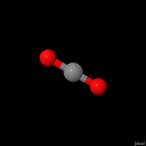
Click on the button below to view and image of the optimized geomtetry of CO₂.
CO₂ is a linear molecule with two C-O bonds each with a length of 1.16 angstroms and a O-O bond with a length of 2.32 angstroms.  By clicking the button bellow you will be able to view an image of the optimized geometry for CO₂ along with its bond lengths measured in angstroms. 
The experimental bond lengths for the C-O bonds were found to be 1.162 angstroms for both on them, and the O-O bond length was found to be 2.324 angstroms.  The experimental values were found on the NIST website.  As you can see the calculated values are very similar to the experimental values, with only a difference of about 0.2% for both the C-O and the O-O bonds. The reason for the O-O bonds is because of pi bonding in the P orbitals between the atoms.  The C-O bond is a sigma bond between the S orbitals of the carbon and oxygen.  Together, these two types of bonds is give CO₂ its double bonds.

Click on the button below to bring up an image of  CO₂'s HOMO, which stands for highest occupied molecular orbial.  Molecular orbitals are defined as the wavefunctions for electrons in the molecule. According to the MacMolPlt program the orbitals displayed are moslty P_z from the two oxygen atoms, and they don't seem to contribute to bonding between the atoms.

CO₂ has three different vibrational modes, with one of them being doubly degenerate.  By clicking the buttons below you will be able to see images of CO₂ vibrating at different frequencies. This is the first vibrational mode for CO₂.  This is one of two degenerate modes. The vibrational frequency calculated was 648.55 cm-1.  It is degenerate because if vibrates at the say frequency even though the atoms are bending in a different direction.  The experimental vibrational frequency is 667.0 cm^-1.  The differenc between the calculated and experimental friquency is about 2.8%.
This the second vibrational mode for CO₂. The vibrational frequency calculated was 1398.15 cm-1.  The experimental values is 1333.0 cm^-1.  The difference between the calculated and experimental frequency is about 4.7%
This the third vibrational mode for CO₂. The vibrational frequency calculated was 2338.18 cm-1.  The experimental frequency found was 2349.0 cm^-1.  The difference between the calculated and experimental frequency is about 0.5%.   

To view and IR spectra of CO₂ follow this link to the NIST website.  As you can see the major peaks in the spectra are between 2200 and 2400 cm^-1 and between 600 and 800 cm^-1.

The table below shows the calculated and experimental dipole moments for CO₂.

Level of Theory	Calculated Dipole Moment (debye)	Experimental Dipole  Moment (debye)
3-21G	0.000010	0.00
6-31G	0.000091	0.00
6-311G	0.000050	0.00

 
All of our calculated results were compared to experimental data found on the NIST website:
http://cccbdb.nist.gov/